Introduction to R

CMOR Lunch’n’Learn

8 March 2023

Ross Wilson

Getting Started

What is R? What is RStudio?

R is a programming language designed to undertake statistical analysis
RStudio is an Integrated Development Environment (IDE) for R
- An IDE is a piece of software including a text editor and other tools to make programming (in this case programming in R, specifically) easier
- You don’t need to use RStudio to use R, but it makes it a lot easier
- To use RStudio, you also need R installed and working

Why learn R?

Powerful and extensible
- Pretty much any statistical analysis you want to do can be done in R
- There are a huge number of freely-available user-written packages that provide all sorts of additional functionality
Reproducibility
- By writing R scripts (code) for your analyses, they can be easily checked/replicated/ updated/adapted, by yourself and others
High-quality graphics
- R has a lot of plotting functions to help you produce publication-quality figures

Getting set up

Install R
- https://cloud.R-project.org/
- Choose the appropriate version for your operating system and follow the instructions
Install RStudio
- https://posit.co/download/rstudio-desktop/
- ditto

Getting to know RStudio

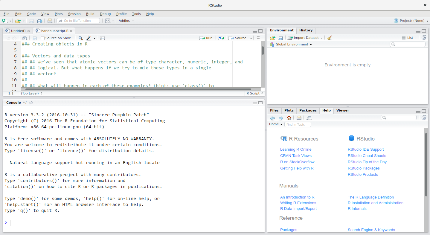
Source

Console

Environment/
History

Files/Plots/
Packages/
Help/Viewer

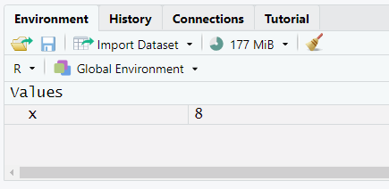
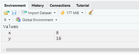
Starting with R

We can type math in the console, and get an answer:

3+5

[1] 8

But to do anything useful, we need to assign the result to a name:

x <- 3 + 5
x

[1] 8

Starting with R

Then we can do things with them:

y <- 2 * x
y

[1] 16

But note that once the value is assigned to y, changing x will not update y:

x <- 25
y

[1] 16

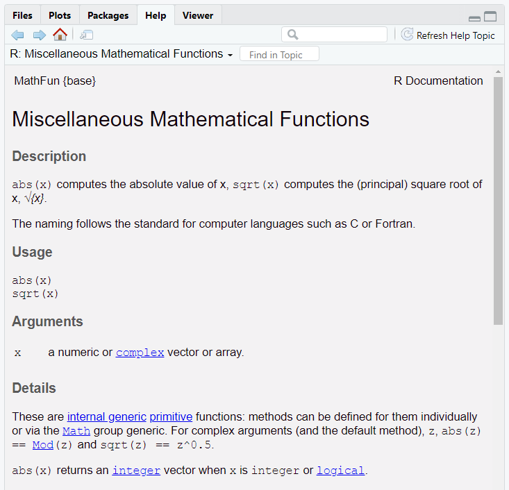
Functions

Functions allow us to run commands other than simple arithmetic

sqrt(x)

[1] 5

Functions consist of a set of input arguments, code that does something with those inputs, and a return value

To get help on a function, look up the documentation

?sqrt

Functions

You can (and should!) also write your own functions

times2 <- function(a) {
    return(a * 2)
}
times2(x)

[1] 50

Separating your code out into discrete functions makes it
- shorter
- easier to follow
- less error prone

Data types

So far we have only seen single numeric values
Data in R can take many forms
- The most basic data structure is the vector

z <- c(3, 7, 10, 6)
z

[1]  3  7 10  6

Vectors can also contain characters

c("apple", "banana")

[1] "apple"  "banana"

The quotes are essential:

otherwise R will look for the names ‘apple’ and ‘banana’ (if these names exist, it will use the values they refer to instead of the character strings; if they don’t, it will give an error)

Data types

The basic data types are numeric, character, logical (TRUE and FALSE values only), and integer
- Also complex and raw, but we don’t need to worry about those
In addition to vectors, more complex data structures include:
- lists: similar to vectors, but the elements can be anything (including other lists), and don’t need to all be the same
- matrices and arrays: like vectors, but with multiple dimensions
- data frames: more on these later

Subsetting

We can extract values from within a vector (or other data structure) with square brackets

a <- c(4, 2, 5, 12)
a[c(4, 2)]

[1] 12  2

a[c(TRUE, FALSE, TRUE, FALSE)]

[1] 4 5

We can use this in conjunction with a logical operator to do conditional subsetting

a[a > 4]

[1]  5 12

Working with Data Frames

Data frames

A data frame is a tabular data structure (like a spreadsheet)
- Each column is a variable
- Each row is an observation
Each column (variable) is a vector, so must contain a single data type
- But different columns can have different types
We can read data from Excel or CSV spreadsheets, data files from Stata etc, previously saved R data frames, and much else…

The `tidyverse`

The ‘tidyverse’ is a collection of packages created by the company that makes RStudio
It contains a lot of functions designed to make working with data frames easier
- tibble: a replacement for base data frames
- readr: read tabular data like csv files (also readxl for Excel files, haven for SPSS/Stata/SAS, and others for different file types)
- dplyr: data manipulation
- tidyr: reshaping and tidying data
- ggplot2: creating plots
- purrr: functional programming
- stringr: working with character strings
- forcats: working with factor variables

Data frames

Reading in a data frame with read_csv():

library(tidyverse)
gapminder <- read_csv("raw_data/gapminder_data.csv")
gapminder

# A tibble: 1,704 × 6
   country      year      pop continent lifeExp gdpPercap
   <chr>       <dbl>    <dbl> <chr>       <dbl>     <dbl>
 1 Afghanistan  1952  8425333 Asia         28.8      779.
 2 Afghanistan  1957  9240934 Asia         30.3      821.
 3 Afghanistan  1962 10267083 Asia         32.0      853.
 4 Afghanistan  1967 11537966 Asia         34.0      836.
 5 Afghanistan  1972 13079460 Asia         36.1      740.
 6 Afghanistan  1977 14880372 Asia         38.4      786.
 7 Afghanistan  1982 12881816 Asia         39.9      978.
 8 Afghanistan  1987 13867957 Asia         40.8      852.
 9 Afghanistan  1992 16317921 Asia         41.7      649.
10 Afghanistan  1997 22227415 Asia         41.8      635.
# ℹ 1,694 more rows

Manipulating data frames with `dplyr`

select() only a subset of variables

select(gapminder, year, country, gdpPercap)

# A tibble: 1,704 × 3
    year country     gdpPercap
   <dbl> <chr>           <dbl>
 1  1952 Afghanistan      779.
 2  1957 Afghanistan      821.
 3  1962 Afghanistan      853.
 4  1967 Afghanistan      836.
 5  1972 Afghanistan      740.
 6  1977 Afghanistan      786.
 7  1982 Afghanistan      978.
 8  1987 Afghanistan      852.
 9  1992 Afghanistan      649.
10  1997 Afghanistan      635.
# ℹ 1,694 more rows

Manipulating data frames with `dplyr`

filter() only a subset of observations

filter(gapminder, continent == "Europe", year == 2007)

# A tibble: 30 × 6
   country                 year      pop continent lifeExp gdpPercap
   <chr>                  <dbl>    <dbl> <chr>       <dbl>     <dbl>
 1 Albania                 2007  3600523 Europe       76.4     5937.
 2 Austria                 2007  8199783 Europe       79.8    36126.
 3 Belgium                 2007 10392226 Europe       79.4    33693.
 4 Bosnia and Herzegovina  2007  4552198 Europe       74.9     7446.
 5 Bulgaria                2007  7322858 Europe       73.0    10681.
 6 Croatia                 2007  4493312 Europe       75.7    14619.
 7 Czech Republic          2007 10228744 Europe       76.5    22833.
 8 Denmark                 2007  5468120 Europe       78.3    35278.
 9 Finland                 2007  5238460 Europe       79.3    33207.
10 France                  2007 61083916 Europe       80.7    30470.
# ℹ 20 more rows

Manipulating data frames with `dplyr`

mutate() to create new variables

mutate(gapminder, gdp_billion = gdpPercap * pop / 10^9)

# A tibble: 1,704 × 7
   country      year      pop continent lifeExp gdpPercap gdp_billion
   <chr>       <dbl>    <dbl> <chr>       <dbl>     <dbl>       <dbl>
 1 Afghanistan  1952  8425333 Asia         28.8      779.        6.57
 2 Afghanistan  1957  9240934 Asia         30.3      821.        7.59
 3 Afghanistan  1962 10267083 Asia         32.0      853.        8.76
 4 Afghanistan  1967 11537966 Asia         34.0      836.        9.65
 5 Afghanistan  1972 13079460 Asia         36.1      740.        9.68
 6 Afghanistan  1977 14880372 Asia         38.4      786.       11.7 
 7 Afghanistan  1982 12881816 Asia         39.9      978.       12.6 
 8 Afghanistan  1987 13867957 Asia         40.8      852.       11.8 
 9 Afghanistan  1992 16317921 Asia         41.7      649.       10.6 
10 Afghanistan  1997 22227415 Asia         41.8      635.       14.1 
# ℹ 1,694 more rows

Manipulating data frames with `dplyr`

summarise() to calculate summary statistics

summarise(gapminder, mean_gdpPercap = mean(gdpPercap))

# A tibble: 1 × 1
  mean_gdpPercap
           <dbl>
1          7215.

This is most useful in conjunction with group_by()

summarise(group_by(gapminder, continent),
                    mean_gdpPercap = mean(gdpPercap))

# A tibble: 5 × 2
  continent mean_gdpPercap
  <chr>              <dbl>
1 Africa             2194.
2 Americas           7136.
3 Asia               7902.
4 Europe            14469.
5 Oceania           18622.

Manipulating data frames with `dplyr`

The power of dplyr is in combining several commands using ‘pipes’
The previous command could be written:

gapminder %>% 
    group_by(continent) %>% 
    summarise(mean_gdpPercap = mean(gdpPercap))

# A tibble: 5 × 2
  continent mean_gdpPercap
  <chr>              <dbl>
1 Africa             2194.
2 Americas           7136.
3 Asia               7902.
4 Europe            14469.
5 Oceania           18622.

Reshaping data frames

Previously we said that data frames have variables in columns and observations in rows
There may be different ways to interpret this in any given dataset
- Our dataset has country-by-year as the observation, and population, life expectancy, and GDP per capita as variables
- Sometimes it might make sense to have one row per country (observation), and multiple variables representing years
- These are known as ‘long’ and ‘wide’ format, respectively

Reshaping data frames

The tidyr package helps us transform our data from one shape to the other
- pivot_wider() takes a long dataset and makes it wider
- pivot_longer() takes a wide dataset and makes it longer
Recall our original dataset

gapminder

# A tibble: 1,704 × 6
   country      year      pop continent lifeExp gdpPercap
   <chr>       <dbl>    <dbl> <chr>       <dbl>     <dbl>
 1 Afghanistan  1952  8425333 Asia         28.8      779.
 2 Afghanistan  1957  9240934 Asia         30.3      821.
 3 Afghanistan  1962 10267083 Asia         32.0      853.
 4 Afghanistan  1967 11537966 Asia         34.0      836.
 5 Afghanistan  1972 13079460 Asia         36.1      740.
 6 Afghanistan  1977 14880372 Asia         38.4      786.
 7 Afghanistan  1982 12881816 Asia         39.9      978.
 8 Afghanistan  1987 13867957 Asia         40.8      852.
 9 Afghanistan  1992 16317921 Asia         41.7      649.
10 Afghanistan  1997 22227415 Asia         41.8      635.
# ℹ 1,694 more rows

Reshaping data frames

We can reshape this to be wider (one row per country)

gapminder_wide <- gapminder %>% 
  pivot_wider(id_cols = c(country, continent),
              names_from = year, values_from = c(pop, lifeExp, gdpPercap))
gapminder_wide

# A tibble: 142 × 38
   country     continent pop_1952 pop_1957 pop_1962 pop_1967 pop_1972 pop_1977
   <chr>       <chr>        <dbl>    <dbl>    <dbl>    <dbl>    <dbl>    <dbl>
 1 Afghanistan Asia       8425333  9240934 10267083 11537966 13079460 14880372
 2 Albania     Europe     1282697  1476505  1728137  1984060  2263554  2509048
 3 Algeria     Africa     9279525 10270856 11000948 12760499 14760787 17152804
 4 Angola      Africa     4232095  4561361  4826015  5247469  5894858  6162675
 5 Argentina   Americas  17876956 19610538 21283783 22934225 24779799 26983828
 6 Australia   Oceania    8691212  9712569 10794968 11872264 13177000 14074100
 7 Austria     Europe     6927772  6965860  7129864  7376998  7544201  7568430
 8 Bahrain     Asia        120447   138655   171863   202182   230800   297410
 9 Bangladesh  Asia      46886859 51365468 56839289 62821884 70759295 80428306
10 Belgium     Europe     8730405  8989111  9218400  9556500  9709100  9821800
# ℹ 132 more rows
# ℹ 30 more variables: pop_1982 <dbl>, pop_1987 <dbl>, pop_1992 <dbl>,
#   pop_1997 <dbl>, pop_2002 <dbl>, pop_2007 <dbl>, lifeExp_1952 <dbl>,
#   lifeExp_1957 <dbl>, lifeExp_1962 <dbl>, lifeExp_1967 <dbl>,
#   lifeExp_1972 <dbl>, lifeExp_1977 <dbl>, lifeExp_1982 <dbl>,
#   lifeExp_1987 <dbl>, lifeExp_1992 <dbl>, lifeExp_1997 <dbl>,
#   lifeExp_2002 <dbl>, lifeExp_2007 <dbl>, gdpPercap_1952 <dbl>, …

Reshaping data frames

Often raw data will come in a wide format, and we want to reshape it longer for data analysis

gapminder_wide %>% 
  pivot_longer(pop_1952:gdpPercap_2007,
               names_to = c(".value", "year"), names_sep = "_")

# A tibble: 1,704 × 6
   country     continent year       pop lifeExp gdpPercap
   <chr>       <chr>     <chr>    <dbl>   <dbl>     <dbl>
 1 Afghanistan Asia      1952   8425333    28.8      779.
 2 Afghanistan Asia      1957   9240934    30.3      821.
 3 Afghanistan Asia      1962  10267083    32.0      853.
 4 Afghanistan Asia      1967  11537966    34.0      836.
 5 Afghanistan Asia      1972  13079460    36.1      740.
 6 Afghanistan Asia      1977  14880372    38.4      786.
 7 Afghanistan Asia      1982  12881816    39.9      978.
 8 Afghanistan Asia      1987  13867957    40.8      852.
 9 Afghanistan Asia      1992  16317921    41.7      649.
10 Afghanistan Asia      1997  22227415    41.8      635.
# ℹ 1,694 more rows

Other `tidyverse` packages

We’ll come back to data visualisation with ggplot2 in a later session
purrr provides tools for functional programming
- If we have several similar datasets, or subgroups within our dataset, we don’t want to write out/copy-and-paste our code separately for each one
- With purrr, we can use map() (and similar) to apply a function to multiple inputs and extract all of the outputs
stringr and forcats are worth looking at if you need to work with string or factor variables – we won’t cover them here

Resources

This material was adapted from the Data Carpentries’ ‘R for Social Scientists’ course (https://preview.carpentries.org/r-socialsci/index.html)
Hands-On Programming with R (https://rstudio-education.github.io/hopr)
- An introduction to programming in R (for non-programmers!)
R for Data Science (https://r4ds.hadley.nz)
- An excellent practical introduction to using the tidyverse
Advanced R (https://adv-r.hadley.nz) and R Packages (https://r-pkgs.org)
- More advanced – good next steps once you’re a bit more comfortable using R

Data analysis in R (regression)

Everything in R is an object

This includes your fitted regression models

Workflow:
- Import/tidy/manipulate raw data
- Run regression or other models
- Use the created model objects
  - print to console
  - save to file
  - extract coefficient estimates
  - plot results
  - export to excel/word
  - etc.

Fitted model objects

R has evolved over time to fit a variety of different needs and use cases
This gives it great flexibility and ability to meet the needs of different users
But, the diversity of interfaces, data structures, implementation, and fitted model objects can be a challenge
- There is often more than one way to fit a given model
- What you’ve learned about one model implemented in a given package may not translate well to working with other functions/packages
We’ll cover some tools to help bridge that gap

Fitted model objects

A few common (but not universal) features:
Models are described by a formula: e.g. y ~ x + z
Data are provided in a data frame (or, equivalently, tibble)
coef(), vcov(), summary() can be used to extract the coefficient estimates, variance covariance matrix, and to print a summary of the fitted model

The `broom` package

broom provides several functions to convert fitted model objects to tidy tibbles
Functions:
- tidy(): construct a tibble that summarises the statistical findings (coefficients, p-values, etc.)
- augment(): add new columns to the original data (predictions/fitted values, etc.)
- glance(): construct a one-row summary of the model (goodness-of-fit, etc.)
The package works with several model fitting functions from base R and commonly-used packages
- Some other packages may also implement their own methods to work with these functions

First example – linear regression

Linear regression models can be fitted with the lm() function (in the stats package, part of base R)
We’ll start by loading the gapminder dataset from the previous session:

library(tidyverse)
gapminder <- read_csv("raw_data/gapminder_data.csv")

First example – linear regression

Use ?lm to find the documentation

linear_regression_model <- lm(lifeExp ~ gdpPercap + continent, gapminder)
linear_regression_model


Call:
lm(formula = lifeExp ~ gdpPercap + continent, data = gapminder)

Coefficients:
      (Intercept)          gdpPercap  continentAmericas  
        4.789e+01          4.453e-04          1.359e+01  
    continentAsia    continentEurope   continentOceania  
        8.658e+00          1.757e+01          1.815e+01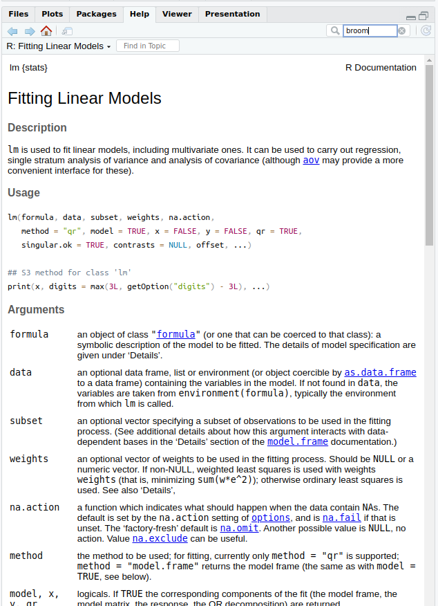

First example – linear regression

linear_regression_model is now a fitted model object
If we want, we can look at how this object is actually stored:

str(linear_regression_model)

List of 13
 $ coefficients : Named num [1:6] 4.79e+01 4.45e-04 1.36e+01 8.66 1.76e+01 ...
  ..- attr(*, "names")= chr [1:6] "(Intercept)" "gdpPercap" "continentAmericas" "continentAsia" ...
 $ residuals    : Named num [1:1704] -28.1 -26.6 -24.9 -22.9 -20.8 ...
  ..- attr(*, "names")= chr [1:1704] "1" "2" "3" "4" ...
 $ effects      : Named num [1:1704] -2455.1 311.1 100.1 -27.9 -223.1 ...
  ..- attr(*, "names")= chr [1:1704] "(Intercept)" "gdpPercap" "continentAmericas" "continentAsia" ...
 $ rank         : int 6
 $ fitted.values: Named num [1:1704] 56.9 56.9 56.9 56.9 56.9 ...
  ..- attr(*, "names")= chr [1:1704] "1" "2" "3" "4" ...
 $ assign       : int [1:6] 0 1 2 2 2 2
 $ qr           :List of 5
  ..$ qr   : num [1:1704, 1:6] -41.2795 0.0242 0.0242 0.0242 0.0242 ...
  .. ..- attr(*, "dimnames")=List of 2
  .. .. ..$ : chr [1:1704] "1" "2" "3" "4" ...
  .. .. ..$ : chr [1:6] "(Intercept)" "gdpPercap" "continentAmericas" "continentAsia" ...
  .. ..- attr(*, "assign")= int [1:6] 0 1 2 2 2 2
  .. ..- attr(*, "contrasts")=List of 1
  .. .. ..$ continent: chr "contr.treatment"
  ..$ qraux: num [1:6] 1.02 1.02 1.01 1.04 1.01 ...
  ..$ pivot: int [1:6] 1 2 3 4 5 6
  ..$ tol  : num 1e-07
  ..$ rank : int 6
  ..- attr(*, "class")= chr "qr"
 $ df.residual  : int 1698
 $ contrasts    :List of 1
  ..$ continent: chr "contr.treatment"
 $ xlevels      :List of 1
  ..$ continent: chr [1:5] "Africa" "Americas" "Asia" "Europe" ...
 $ call         : language lm(formula = lifeExp ~ gdpPercap + continent, data = gapminder)
 $ terms        :Classes 'terms', 'formula'  language lifeExp ~ gdpPercap + continent
  .. ..- attr(*, "variables")= language list(lifeExp, gdpPercap, continent)
  .. ..- attr(*, "factors")= int [1:3, 1:2] 0 1 0 0 0 1
  .. .. ..- attr(*, "dimnames")=List of 2
  .. .. .. ..$ : chr [1:3] "lifeExp" "gdpPercap" "continent"
  .. .. .. ..$ : chr [1:2] "gdpPercap" "continent"
  .. ..- attr(*, "term.labels")= chr [1:2] "gdpPercap" "continent"
  .. ..- attr(*, "order")= int [1:2] 1 1
  .. ..- attr(*, "intercept")= int 1
  .. ..- attr(*, "response")= int 1
  .. ..- attr(*, ".Environment")=<environment: R_GlobalEnv> 
  .. ..- attr(*, "predvars")= language list(lifeExp, gdpPercap, continent)
  .. ..- attr(*, "dataClasses")= Named chr [1:3] "numeric" "numeric" "character"
  .. .. ..- attr(*, "names")= chr [1:3] "lifeExp" "gdpPercap" "continent"
 $ model        :'data.frame':  1704 obs. of  3 variables:
  ..$ lifeExp  : num [1:1704] 28.8 30.3 32 34 36.1 ...
  ..$ gdpPercap: num [1:1704] 779 821 853 836 740 ...
  ..$ continent: chr [1:1704] "Asia" "Asia" "Asia" "Asia" ...
  ..- attr(*, "terms")=Classes 'terms', 'formula'  language lifeExp ~ gdpPercap + continent
  .. .. ..- attr(*, "variables")= language list(lifeExp, gdpPercap, continent)
  .. .. ..- attr(*, "factors")= int [1:3, 1:2] 0 1 0 0 0 1
  .. .. .. ..- attr(*, "dimnames")=List of 2
  .. .. .. .. ..$ : chr [1:3] "lifeExp" "gdpPercap" "continent"
  .. .. .. .. ..$ : chr [1:2] "gdpPercap" "continent"
  .. .. ..- attr(*, "term.labels")= chr [1:2] "gdpPercap" "continent"
  .. .. ..- attr(*, "order")= int [1:2] 1 1
  .. .. ..- attr(*, "intercept")= int 1
  .. .. ..- attr(*, "response")= int 1
  .. .. ..- attr(*, ".Environment")=<environment: R_GlobalEnv> 
  .. .. ..- attr(*, "predvars")= language list(lifeExp, gdpPercap, continent)
  .. .. ..- attr(*, "dataClasses")= Named chr [1:3] "numeric" "numeric" "character"
  .. .. .. ..- attr(*, "names")= chr [1:3] "lifeExp" "gdpPercap" "continent"
 - attr(*, "class")= chr "lm"

First example – linear regression

More usefully, we can print a summary of the model

summary(linear_regression_model)


Call:
lm(formula = lifeExp ~ gdpPercap + continent, data = gapminder)

Residuals:
    Min      1Q  Median      3Q     Max 
-49.241  -4.479   0.347   5.105  25.138 

Coefficients:
                   Estimate Std. Error t value Pr(>|t|)    
(Intercept)       4.789e+01  3.398e-01  140.93   <2e-16 ***
gdpPercap         4.453e-04  2.350e-05   18.95   <2e-16 ***
continentAmericas 1.359e+01  6.008e-01   22.62   <2e-16 ***
continentAsia     8.658e+00  5.555e-01   15.59   <2e-16 ***
continentEurope   1.757e+01  6.257e-01   28.08   <2e-16 ***
continentOceania  1.815e+01  1.787e+00   10.15   <2e-16 ***
---
Signif. codes:  0 '***' 0.001 '**' 0.01 '*' 0.05 '.' 0.1 ' ' 1

Residual standard error: 8.39 on 1698 degrees of freedom
Multiple R-squared:  0.5793,    Adjusted R-squared:  0.5781 
F-statistic: 467.7 on 5 and 1698 DF,  p-value: < 2.2e-16

First example – linear regression

If we want to work with the results or combine/compare them with other models, tidy() from the broom package will put them into a nice tidy tibble

library(broom)
tidy(linear_regression_model)

# A tibble: 6 × 5
  term               estimate std.error statistic   p.value
  <chr>                 <dbl>     <dbl>     <dbl>     <dbl>
1 (Intercept)       47.9      0.340         141.  0        
2 gdpPercap          0.000445 0.0000235      18.9 8.55e- 73
3 continentAmericas 13.6      0.601          22.6 2.82e- 99
4 continentAsia      8.66     0.555          15.6 2.72e- 51
5 continentEurope   17.6      0.626          28.1 7.60e-143
6 continentOceania  18.1      1.79           10.2 1.50e- 23

And glance() gives us several overall model statistics

glance(linear_regression_model)

# A tibble: 1 × 12
  r.squared adj.r.squared sigma statistic   p.value    df logLik    AIC    BIC deviance
      <dbl>         <dbl> <dbl>     <dbl>     <dbl> <dbl>  <dbl>  <dbl>  <dbl>    <dbl>
1     0.579         0.578  8.39      468. 4.26e-316     5 -6039. 12093. 12131.  119528.
# ℹ 2 more variables: df.residual <int>, nobs <int>

First example – linear regression

The lmtest and car packages provide tools for inference & hypothesis testing
Various clustered and heteroskedasticity-robust standard errors are provided by sandwich
- These work well together (and with tidy() from broom)

library(lmtest)
library(sandwich)
linear_regression_model %>% 
  coeftest(vcov. = vcovCL, cluster = ~country) %>% 
    tidy()

# A tibble: 6 × 5
  term               estimate std.error statistic  p.value
  <chr>                 <dbl>     <dbl>     <dbl>    <dbl>
1 (Intercept)       47.9       0.904        53.0  0       
2 gdpPercap          0.000445  0.000159      2.81 5.05e- 3
3 continentAmericas 13.6       1.56          8.69 8.32e-18
4 continentAsia      8.66      1.55          5.57 2.98e- 8
5 continentEurope   17.6       2.18          8.06 1.44e-15
6 continentOceania  18.1       2.77          6.55 7.36e-11

Generalised linear regression

Can be fitted with the glm() function
(also in the stats package)

?glm

gen_linear_regression_model <- glm(lifeExp ~ gdpPercap + continent,
                                   family = "quasipoisson", gapminder)
gen_linear_regression_model


Call:  glm(formula = lifeExp ~ gdpPercap + continent, family = "quasipoisson", 
    data = gapminder)

Coefficients:
      (Intercept)          gdpPercap  continentAmericas  
        3.875e+00          6.156e-06          2.490e-01  
    continentAsia    continentEurope   continentOceania  
        1.671e-01          3.092e-01          3.177e-01  

Degrees of Freedom: 1703 Total (i.e. Null);  1698 Residual
Null Deviance:      4946 
Residual Deviance: 2229     AIC: NA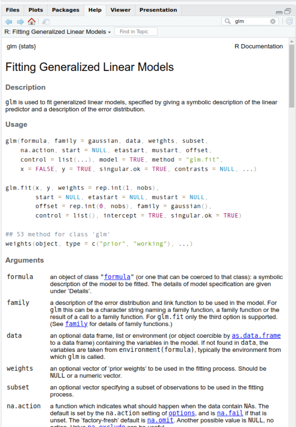

Generalised linear regression

Again, we can print a summary of the model

summary(gen_linear_regression_model)


Call:
glm(formula = lifeExp ~ gdpPercap + continent, family = "quasipoisson", 
    data = gapminder)

Coefficients:
                   Estimate Std. Error t value Pr(>|t|)    
(Intercept)       3.875e+00  6.524e-03  594.03   <2e-16 ***
gdpPercap         6.156e-06  3.475e-07   17.72   <2e-16 ***
continentAmericas 2.490e-01  1.054e-02   23.62   <2e-16 ***
continentAsia     1.671e-01  1.009e-02   16.55   <2e-16 ***
continentEurope   3.092e-01  1.054e-02   29.33   <2e-16 ***
continentOceania  3.177e-01  2.815e-02   11.29   <2e-16 ***
---
Signif. codes:  0 '***' 0.001 '**' 0.01 '*' 0.05 '.' 0.1 ' ' 1

(Dispersion parameter for quasipoisson family taken to be 1.279258)

    Null deviance: 4945.6  on 1703  degrees of freedom
Residual deviance: 2229.4  on 1698  degrees of freedom
AIC: NA

Number of Fisher Scoring iterations: 4

Generalised linear regression

And use tidy() and glance() from the broom package to produce nice tidy tibbles

tidy(gen_linear_regression_model, conf.int = TRUE, exponentiate = TRUE)

# A tibble: 6 × 7
  term              estimate   std.error statistic   p.value conf.low conf.high
  <chr>                <dbl>       <dbl>     <dbl>     <dbl>    <dbl>     <dbl>
1 (Intercept)          48.2  0.00652         594.  0            47.6      48.8 
2 gdpPercap             1.00 0.000000347      17.7 1.42e- 64     1.00      1.00
3 continentAmericas     1.28 0.0105           23.6 6.86e-107     1.26      1.31
4 continentAsia         1.18 0.0101           16.6 3.57e- 57     1.16      1.21
5 continentEurope       1.36 0.0105           29.3 2.32e-153     1.33      1.39
6 continentOceania      1.37 0.0282           11.3 1.57e- 28     1.30      1.45

glance(gen_linear_regression_model)

# A tibble: 1 × 8
  null.deviance df.null logLik   AIC   BIC deviance df.residual  nobs
          <dbl>   <int>  <dbl> <dbl> <dbl>    <dbl>       <int> <int>
1         4946.    1703     NA    NA    NA    2229.        1698  1704

What else?

There are many (many!) other packages that estimate different regression models or provide tools for diagnostic testing, post-hoc analysis, or visualisation of regression models
For example, the Econometrics Task View on cran.r-project.org

Some that might be of particular relevance to (some of) you:
- mediation: parametric and non-parametric mediation analysis
- eRm and ltm: Rasch models
- metafor: meta-analysis
- rstan, rstanarm, and brms: Bayesian analysis (using Stan)
- plm, fixest, lme4, and nlme: panel and multi-level/mixed effect models

Data visualisation

Data visualisation with `ggplot2`

There are a lot of tools available to create plots in R
- ggplot2 is the most well-developed and widely used
We generally want data in long format for plotting
- One column for each variable
- One row for each observation
We’ll use the gapminder dataset from the previous session

library(tidyverse)
gapminder <- read_csv("raw_data/gapminder_data.csv")

The grammar of graphics

dataset – self-explanatory
geom – the geometric object used to represent the data
mappings – which features of the geom represent which variables in the data
stats – transformations of the data before plotting
position – to avoid overplotting data points
coordinate system – how the x and y axes are plotted
faceting scheme – split the plot by subgroups

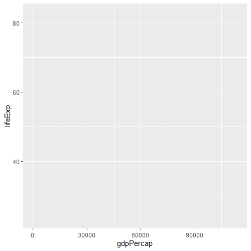
Data visualisation with `ggplot2`

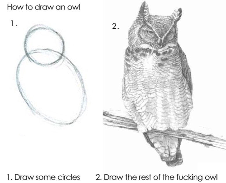
That’s the theory
In practice, the easiest way is to build the plot up step-by-step (trial-and-error)
- start with the basic ggplot object

ggplot(data = gapminder)

you can specify (some of) the mappings at this stage

ggplot(data = gapminder, mapping = aes(x = gdpPercap, y = lifeExp))

Data analysis workflows and project organisation

Reproducible research

What is ‘reproducibility’?
- Focus here is on computational reproducibility – can your results be replicated by someone (or yourself!) with access to your data, code, etc.
Why might research not be reproducible?
- Raw data are not available or have been changed
- Intermediate steps taken to extract, clean, reshape, merge, or analyse data are not adequately recorded or described
- Software tools have changed or are no longer available since the analysis was conducted
- Errors in manually transcribing results from analysis software to final report (manuscript, etc.)

Reproducible research

Computers are now essential in all branches of science, but most researchers are never taught the equivalent of basic lab skills for research computing. As a result, data can get lost, analyses can take much longer than necessary, and researchers are limited in how effectively they can work with software and data. Computing workflows need to follow the same practices as lab projects and notebooks, with organized data, documented steps, and the project structured for reproducibility, but researchers new to computing often don’t know where to start.

— Wilson G, Bryan J, Cranston K, et al. Good enough practices in scientific computing. PLoS Comput Biol 2017;13:e1005510

Reproducible research

Ensuring reproducibility (for others) can also have great benefits for you as the analyst/author
- When you come back to an analysis later, you know exactly what you did, why you did it, and how to replicate it if needed
- If data changes, errors are identified, or new analyses need to be conducted, your analysis and results can easily be updated
- The code and methods used in one project/analysis can be re-used in other work
- Keeping to a simple, standardised workflow for all projects allows you to switch easily & quickly between projects
  - And prevents you having to make a whole bunch of new decisions every time you start something new

Key principles

Raw data stays raw
Source is real
Design for collaboration
- (including with your future self)
Consider version control
Automation?

Key principles – Raw data

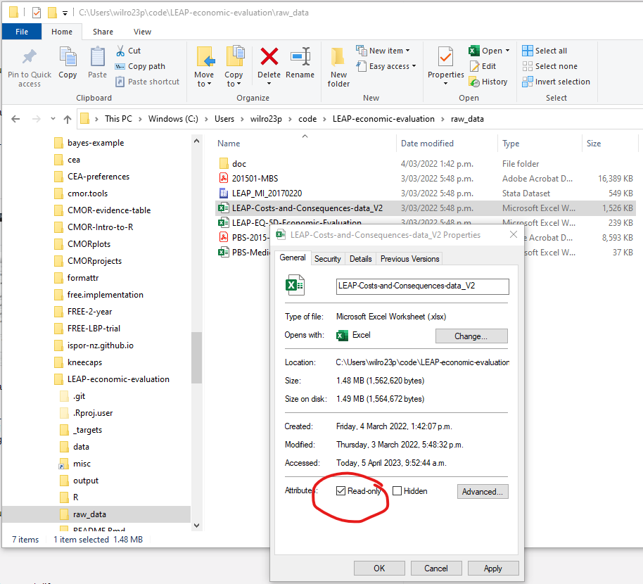
Raw data stays raw
- Make raw data files read-only

Key principles – Raw data

Raw data stays raw
- Make raw data files read-only
- Can be relaxed (temporarily) if needed, but avoids accidental changes
- Most (probably all) changes to data should be scripted (in R, Stata, etc.) rather than made directly in raw data files

Key principles

Raw data stays raw
Source is real
Design for collaboration
- (including with your future self)
Consider version control
Automation?

Key principles

Raw data stays raw
Source is real
Design for collaboration
- (including with your future self)
Consider version control
Automation?

Key principles – Source files

Source is real…
- …workspace is replaceable
Any individual R session is disposable and can be replaced/recreated at any time, if you have raw data and appropriate source code
Thinking in this way forces you to follow good reproducibility practices in your analysis workflow

Key principles – Source files

What does ‘Source is real’ mean?
- Data import, cleaning, reshaping, wrangling, and analysis should all be conducted via script files
  - or at least documented in thorough, step-by-step detail
- All source code should be saved (regularly!) so all of these steps can be reproduced at any time
- Important (or time-consuming) intermediate objects (cleaned datasets, figures, etc) should be explicitly saved, individually, to files (by script, not the mouse, if possible)

Key principles – Source files

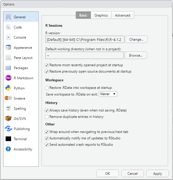
Start R with a blank slate, and restart often

Key principles – Source files

Start R with a blank slate, and restart often
- When you are running code interactively to try things out, you will be adding objects to the workspace, loading packages, etc
- If you inadvertently rely on these objects, packages, etc in your source files, you may not be able to reproduce your results in a new session later
- If you have saved source code and intermediate objects to file as you go, it is quick and easy to restart R (Ctrl+Shift+F10, in RStudio) regularly to check whether everything still works as expected
  - It is much better to find this out after a few minutes than after a whole day’s work!

Key principles

Raw data stays raw
Source is real
Design for collaboration
- (including with your future self)
Consider version control
Automation?

Key principles

Raw data stays raw
Source is real
Design for collaboration
- (including with your future self)
Consider version control
Automation?

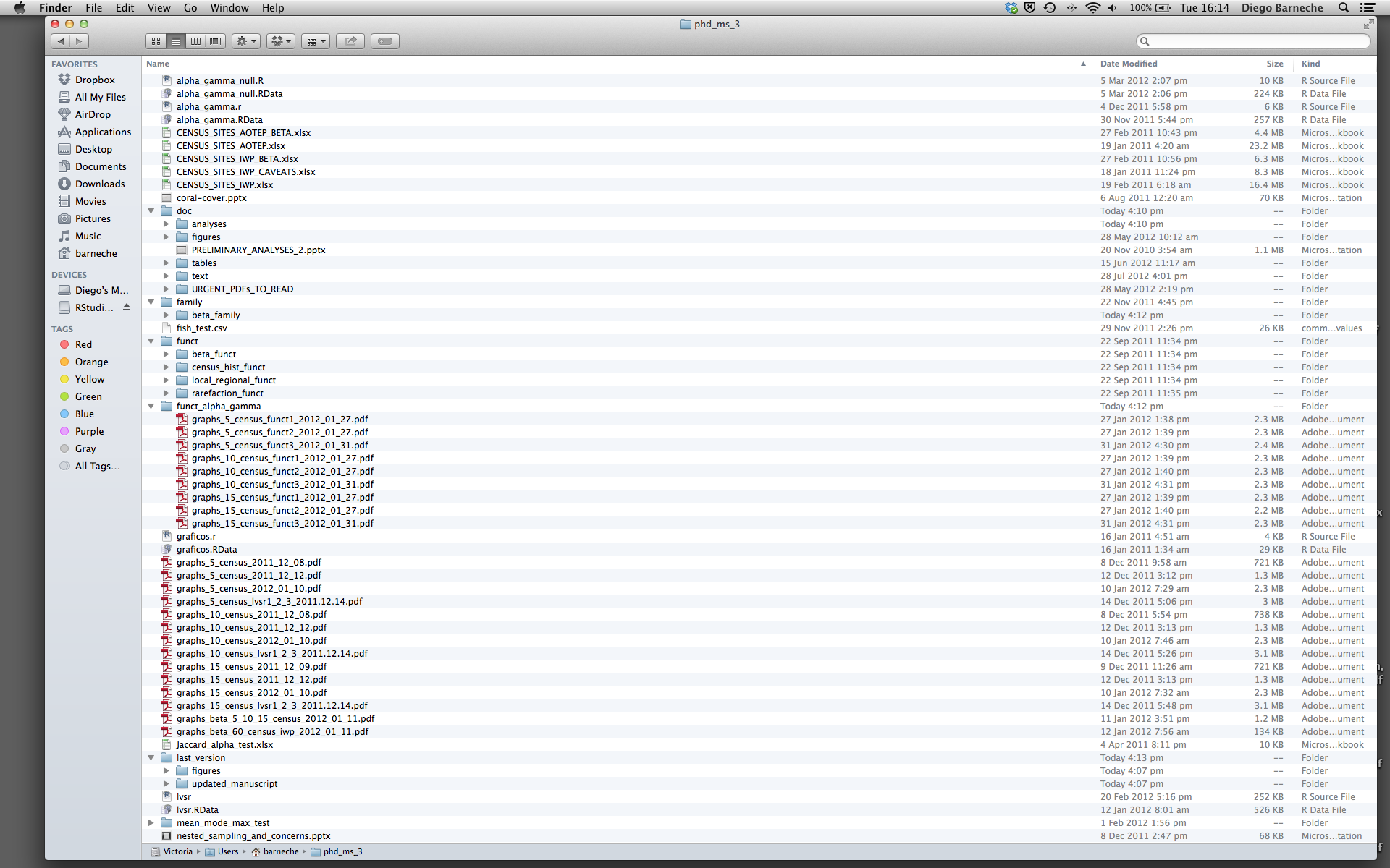
Key principles – Design for collaboration

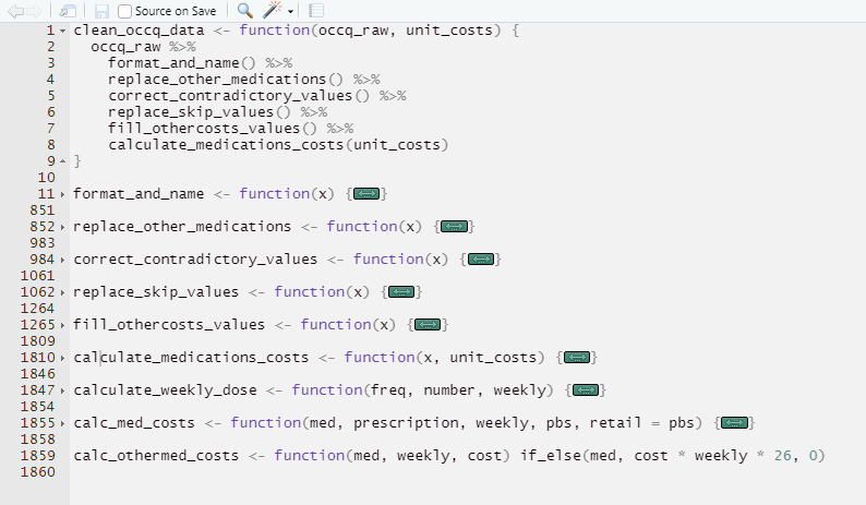
An analysis directory like this makes it very difficult for anyone (including yourself later) to follow the steps required to reproduce your results

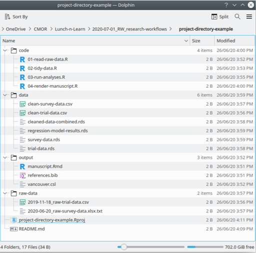
Key principles – Design for collaboration

Much better to follow a logical structure (and the same across all of your projects)
- Set out high-level structure, e.g.
  1. read raw data
  2. tidy data for analysis
  3. run analyses on tidy data
  4. collate report/results of analyses
- Put raw data in its own directory (and read-only)
- Consider other structures/subfolders as appropriate for your project

Key principles – Design for collaboration

Break up complicated or repeated analysis steps into discrete functions
Give functions and variables meaningful names
Use comments liberally

Key principles

Raw data stays raw
Source is real
Design for collaboration
- (including with your future self)
Consider version control
Automation?

Key principles

Raw data stays raw
Source is real
Design for collaboration
- (including with your future self)
Consider version control
Automation?

Key principles – Version control

Keeping track of changes to data and code (and being able to revert to a previous version if things go wrong) is critical for reproducible research
This is particularly true when collaborating with others
The best way to do this is with a version control system such as Git

Key principles – Version control

We won’t go into this in detail today, but a quick Getting Started guide:
- Register a GitHub account (https://github.com)
- Install Git (https://git-scm.com) and complete basic setup
- Get a Git client (GUI)
  - GitKraken is a good choice (https://gitkraken.com)
  - GitHub offers a free client, GitHub Desktop (https://desktop.github.com/)
  - RStudio has a basic Git client built-in, which is fine for much day-to-day use
See https://happygitwithr.com/ for more detailed instructions

Key principles – Version control

Using Git (& GitHub) in your projects
- A couple of ways to get this set up. Probably the easiest is:
- Create a project repository (repo) on GitHub
- Import (‘clone’) the repo as a new RStudio project
- Make changes as usual in RStudio (or any other program)
- ‘Commit’ (take a snapshot of the current state of the project) often to your local repo
- Less often (maybe once/day) ‘push’ (sync) the local repo to GitHub
What to put under version control
- Source code
- Raw data (unless its very large)

What not to put under version control

Most intermediate objects
Miscellaneous supporting documents (pdf files, etc.)
Final output in the form of word documents, etc.

Key principles

Raw data stays raw
Source is real
Design for collaboration
- (including with your future self)
Consider version control
Automation?

Key principles

Raw data stays raw
Source is real
Design for collaboration
- (including with your future self)
Consider version control
Automation?

Key principles – Automation

Just as we treat source code as the ‘true’, reproducible record of each step of the analysis, we can record (and automate) how the sequence of individual steps fits together to produce our final results

Can be as simple as something like:

source("code/00-download-data.R")
source("code/01-tabulate-frequencies.R")
source("code/02-create-histogram.R")
source("code/03-render-report.R")

Shows in what order to run the scripts, and allows us to resume from the middle (if, for example, you have only changed the file 02-create-histogram.R, there is no need to redo the first two steps, but we do need to rerun the create-histogram and render-report steps
- Each script should load the required inputs and save the resulting output to file

Key principles – Automation

For more complicated (or long-running) analyses, we may want to explicitly specify dependencies and let the computer figure out how to get everything up-to-date
Two good tools for doing this:
- make
- targets
Advantages of an automated pipeline like this:
- When you modify one stage of the pipeline, you can re-run your analyses to get up-to-date final results, with a single click/command
- Only the things that need to be updated will be re-run, saving time (important if some of your analyses take a long time to run)

Key principles – Automation

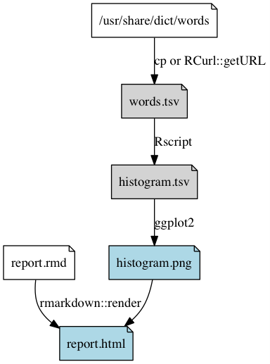
Make is a system tool, designed for use in software development, to specify targets, commands, and dependencies between files and selectively re-run commands when dependencies change
A Makefile is a plain text file specifying a list of these targets (intermediate/output files in the analysis workflow), commands (to create the targets), and dependencies (input files needed for each command)

words.txt: /usr/share/dict/words
    cp /usr/share/dict/words words.txt

histogram.tsv: histogram.r words.txt
    Rscript $<

histogram.png: histogram.tsv
    Rscript -e 'library(ggplot2); qplot(Length, Freq, data=read.delim("$<")); ggsave("$@")'

report.html: report.rmd histogram.tsv histogram.png
    Rscript -e 'rmarkdown::render("$<")'

Key principles – Automation

targets is an R package designed to do something very similar, but specifically designed for R projects

plan <- list(
  tar_file(words, download_words()),
  tar_target(frequency_table, summarise_word_lengths(words)),
  tar_target(histogram, create_histogram(frequency_table)),
  tar_file(report, render_report("reports/report.rmd", frequency_table, histogram))
)

Abstract workflow steps behind function calls (with meaningful names) as much as possible
- The plan should be a clear, high-level overview of the analysis steps required

Summary

Treat raw data as read-only
Save source, not the workspace
Design for collaboration
- Follow a logical project structure
- Simplify code with human-readable abstractions (functions etc)
Consider version control
Consider automating your analyses

Summary

Treat raw data as read-only
Save source, not the workspace
Design for collaboration
- Follow a logical project structure
- Simplify code with human-readable abstractions (functions etc)
Consider version control
Consider automating your analyses

(if you are already writing
script files for your analyses)

(will get better
with practice)

(start with a simple high-level overview of the steps in the analysis,
even if you don’t want to do a full automated pipeline)

Resources

Wilson G, Aruliah DA, Brown CT, Chue Hong NP, Davis M, et al. (2014) Best Practices for Scientific Computing. PLoS Biol 12(1):e1001745. https://doi.org/10.1371/journal.pbio.1001745
Wilson G, Bryan J, Cranston K, Kitzes J, Nederbragt L, Teal TK (2017) Good enough practices in scientific computing. PloS Comput Biol 13(6):e1005510. https://doi.org/10.1371/journal.pcbi.1005510
Bryan J, Hester J. What they forgot to teach you about R. https://rstats.wtf (especially Section I: A holistic workflow)
Bryan J. STAT545 (based on the UBC course of the same name). https://stat545.com
Bryan J. Happy Git and GitHub for the useR. https://happygitwithr.com
For targets:
- McBain M. Benefits of a function-based diet (The {drake} post). https://milesmcbain.xyz/the-drake-post/
  - Refers to the drake package, which was a predecessor package of targets. The same concepts all apply
- Landau W. The {targets} R package user manual. https://books.ropensci.org/targets/

Writing reports in R

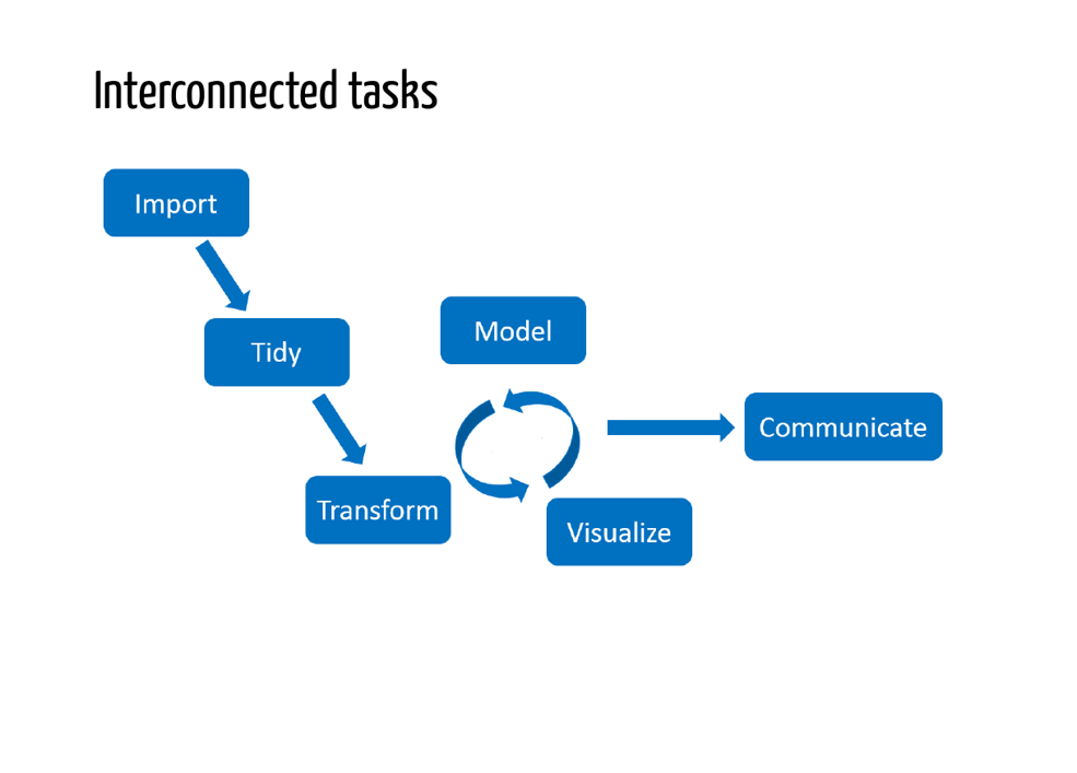
Data workflow

plan <- list(
  tar_file(words, download_words()),
  tar_target(frequency_table, summarise_word_lengths(words)),
  tar_target(histogram, create_histogram(frequency_table)),
  tar_file(report, render_report("reports/report.rmd", frequency_table, histogram))
)

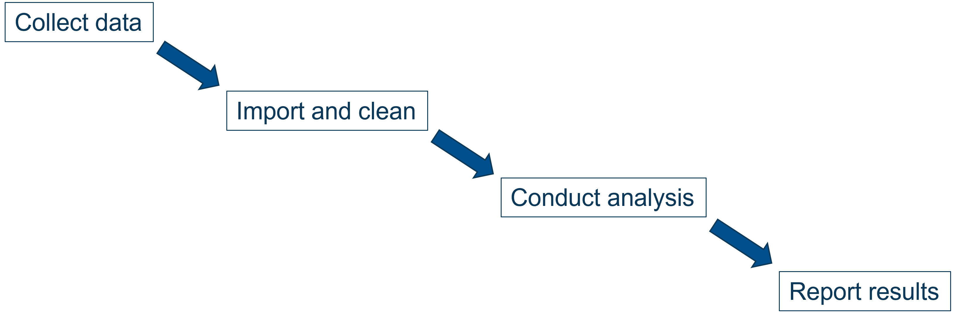
Advantages:

Reported results are always kept up-to-date with data and analysis
Changes at any point along the workflow can be made easily and robustly

Data workflow

plan <- list(
  tar_file(words, download_words()),
  tar_target(frequency_table, summarise_word_lengths(words)),
  tar_target(histogram, create_histogram(frequency_table)),
  tar_file(report, render_report("reports/report.rmd", frequency_table, histogram))
)

Advantages:

Reported results are always kept up-to-date with data and analysis
Changes at any point along the workflow can be made easily and robustly

R Markdown

Quarto

We’ll focus on Quarto instead
Quarto is a relatively new tool very similar to RMarkdown
- Most of what you might read about RMarkdown also applies to Quarto
- see also https://quarto.org for documentation and guides

Introduction to R

Getting Started

What is R? What is RStudio?

Why learn R?

Getting set up

Getting to know RStudio

Starting with R

Starting with R

Functions

Functions

Data types

Data types

Subsetting

Working with Data Frames

Data frames

The tidyverse

Data frames

Manipulating data frames with dplyr

Manipulating data frames with dplyr

Manipulating data frames with dplyr

Manipulating data frames with dplyr

Manipulating data frames with dplyr

Reshaping data frames

Reshaping data frames

Reshaping data frames

Reshaping data frames

Other tidyverse packages

Resources

Data analysis in R (regression)

Everything in R is an object

Fitted model objects

Fitted model objects

The broom package

First example – linear regression

First example – linear regression

First example – linear regression

First example – linear regression

First example – linear regression

First example – linear regression

Generalised linear regression

Generalised linear regression

Generalised linear regression

What else?

Data visualisation

Data visualisation with ggplot2

The grammar of graphics

Data visualisation with ggplot2

Data analysis workflows and project organisation

Reproducible research

Reproducible research

Reproducible research

Key principles

Key principles – Raw data

Key principles – Raw data

Key principles – Raw data

Key principles

Key principles

Key principles – Source files

Key principles – Source files

Key principles – Source files

Key principles – Source files

Key principles – Source files

Key principles

Key principles

Key principles – Design for collaboration

Key principles – Design for collaboration

Key principles – Design for collaboration

Key principles

Key principles

Key principles – Version control

Key principles – Version control

Key principles – Version control

Key principles

Key principles

Key principles – Automation

Key principles – Automation

Key principles – Automation

Key principles – Automation

Summary

Summary

The `tidyverse`

Manipulating data frames with `dplyr`

Manipulating data frames with `dplyr`

Manipulating data frames with `dplyr`

Manipulating data frames with `dplyr`

Manipulating data frames with `dplyr`

Other `tidyverse` packages

The `broom` package

Data visualisation with `ggplot2`

Data visualisation with `ggplot2`